Constructing Histograms with matplotlib.pyplot.hist

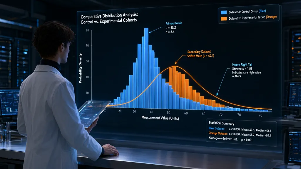
A histogram is only as honest as its bins. Too few bins can bury a second peak or a long tail; too many can turn ordinary sampling noise into a flock of apparent structure. Choose the bin width to answer a specific question, not to make the plot look busy.

For a first pass, let the data suggest a width. NumPy’s Freedman–Diaconis rule uses the interquartile range, so a handful of extreme values has less influence than it would with a standard-deviation-based rule:

import numpy as np
import matplotlib.pyplot as plt

values = np.asarray(values)
values = values[np.isfinite(values)]

fig, ax = plt.subplots()
ax.hist(values, bins="fd", edgecolor="white")

The rule is a useful default, not a verdict. If the sample is small, the distribution is highly discrete, or the result will be compared with another dataset, an explicit bin width is often easier to interpret and reproduce. For example, measurements recorded to the nearest tenth should not be shown with bins far narrower than a tenth.

width = 0.5
edges = np.arange(values.min(), values.max() + width, width)

fig, ax = plt.subplots()
ax.hist(values, bins=edges, edgecolor="white")

When several plots need direct comparison, use the same edges for every dataset. Letting each histogram choose its own bins can make identical patterns look different, or different patterns look deceptively similar.

edges = np.linspace(0, 100, 21)

fig, ax = plt.subplots()
ax.hist(group_a, bins=edges, alpha=0.55, label="A")
ax.hist(group_b, bins=edges, alpha=0.55, label="B")
ax.legend()

For a skewed distribution spanning orders of magnitude, equal-width bins may waste most of the plot on a sparse tail. Log-spaced edges can show the shape across scales, but only positive values belong in such bins:

positive = values[values > 0]
edges = np.geomspace(positive.min(), positive.max(), 25)

fig, ax = plt.subplots()
ax.hist(positive, bins=edges, edgecolor="white")
ax.set_xscale("log")

Inspect the edges as well as the bars. A bin boundary placed on a meaningful threshold can split values that should be treated together; shifting the edges can reveal whether a striking feature is genuine or merely an artifact of where the bins fell.

Feed hist into the plotting pipeline

Axes.hist is the convenient path from samples to bars: it bins the values and draws the result on the supplied axes. Keep the axes object explicit, especially in scripts that create several plots, rather than relying on pyplot’s current-figure state.

fig, ax = plt.subplots()
counts, edges, bars = ax.hist(values, bins=edges, edgecolor="white")
ax.set_xlabel("Latency (ms)")
ax.set_ylabel("Observations")

The return values are useful when the plot is only one stage in a larger pipeline. counts contains the bin totals, edges the boundaries used, and bars the Matplotlib artists. Pass those totals to later calculations or tests instead of trying to recover them from the rendered rectangles.

counts, edges = np.histogram(values, bins=edges)

fig, ax = plt.subplots()
ax.stairs(counts, edges, fill=True, alpha=0.7)

This separation is handy when binning and presentation have different responsibilities: NumPy computes the histogram, while Matplotlib draws it. The same counts and edges can also be saved, compared, or rendered with a different style without repeating the binning step.

For several datasets, Axes.hist accepts a sequence of arrays. Supply shared edges so each series refers to the same intervals, and choose an arrangement that matches the comparison: overlapping bars expose relative shape, while stacked bars emphasize the combined total.

fig, ax = plt.subplots()
ax.hist(
    [group_a, group_b],
    bins=edges,
    label=["A", "B"],
    alpha=0.6,
    histtype="stepfilled",
)
ax.legend()

If the sample is already summarized as counts, do not expand each bin into repeated observations just to call hist. Draw the bins directly with stairs; it accepts one value per interval and the corresponding sequence of edges.

Normalize counts when comparisons matter

Raw counts answer “how many observations fell here?” They also rise with sample size, so a larger dataset can produce taller bars even when its distribution has the same shape. For shape comparisons across samples of different sizes, normalize each histogram to unit area:

fig, ax = plt.subplots()
ax.hist(group_a, bins=edges, density=True, alpha=0.5, label="A")
ax.hist(group_b, bins=edges, density=True, alpha=0.5, label="B")
ax.set_ylabel("Probability density")
ax.legend()

With density=True, bar heights are densities, not probabilities. The area of each bar is its height multiplied by its bin width, and the areas across all bins sum to one. This distinction matters when bins have unequal widths: a tall, narrow bar may represent fewer observations than a shorter, wide one.

density, edges = np.histogram(values, bins=edges, density=True)
probability_per_bin = density * np.diff(edges)

assert np.isclose(probability_per_bin.sum(), 1.0)

If the bins have equal widths, dividing counts by the total gives the fraction of observations in each bin. Those fractions are often easier to explain than densities when the intended quantity is “share of the sample in this interval.”

counts, edges = np.histogram(values, bins=edges)
fractions = counts / counts.sum()

fig, ax = plt.subplots()
ax.stairs(fractions, edges, fill=True, alpha=0.7)
ax.set_ylabel("Fraction of observations")

Do not confuse normalization with equalizing every bin. Unit-area normalization preserves the shape and relative concentration of the data; it only removes the effect of total sample size. If the question is instead about absolute volume, retain counts and make the sample sizes explicit.

Weights provide another normalization path when each observation represents a different amount. For example, survey records may carry sampling weights. Normalize the weighted sum in each bin to obtain a weighted density, and use the same interpretation consistently across datasets.

weights = np.asarray(weights, dtype=float)

fig, ax = plt.subplots()
ax.hist(
    values,
    bins=edges,
    weights=weights,
    density=True,
    edgecolor="white",
)
ax.set_ylabel("Weighted probability density")

Check what the denominator means before comparing normalized plots. Each histogram normalized independently describes its own sample’s shape; it no longer communicates the relative size of the samples. When both shape and sample size matter, show normalized distributions alongside the sample counts, or use separate panels with a shared bin definition.

Tune labels, limits, and appearance

Labels should name both the quantity and its units. “Count” is better than no y-axis label; “Latency (ms)” is better than “Value.” If the bars show density or fractions, say so explicitly: the height then has a different meaning from a raw observation count.

fig, ax = plt.subplots()
ax.hist(values, bins=edges, edgecolor="white", color="steelblue")
ax.set_xlabel("Latency (ms)")
ax.set_ylabel("Observations")
ax.set_title("Request latency")

Set limits only when the bounds serve a purpose. A zero lower bound is often appropriate for counts, while a measurement axis may need a narrower range to expose variation. Clipping data can hide outliers without warning, so report the displayed range and check how many observations fall outside it.

low, high = 0, 500
outside = np.count_nonzero((values < low) | (values > high))

fig, ax = plt.subplots()
ax.hist(values, bins=edges, edgecolor="white")
ax.set_xlim(low, high)
print(f"{outside} observations fall outside the displayed range")

For a long-tailed distribution, a logarithmic x-axis can make small values legible alongside large ones, but it does not change the bin counts already computed. Use positive, logarithmically spaced bin edges when the bins themselves should represent equal multiplicative intervals.

positive = values[values > 0]
edges = np.geomspace(positive.min(), positive.max(), 25)

fig, ax = plt.subplots()
ax.hist(positive, bins=edges, edgecolor="white")
ax.set_xscale("log")
ax.set_xlabel("Size (bytes, logarithmic scale)")
ax.set_ylabel("Observations")

Use ticks that help readers estimate values without turning the axes into a second data display. For a known scale, choose a deliberate interval; for irregular bin edges, avoid labeling every edge if the labels collide.

fig, ax = plt.subplots()
ax.hist(values, bins=edges, edgecolor="white")
ax.set_xticks(np.arange(0, 101, 20))
ax.grid(axis="y", alpha=0.25)
ax.set_axisbelow(True)

Keep visual emphasis subordinate to the distribution. A light edge separates adjacent bars; a restrained grid helps estimate heights. When datasets overlap, transparency can reveal both, but too many opaque colors quickly obscure the counts. A step histogram is often clearer for several series sharing the same bins.

fig, ax = plt.subplots()
ax.hist(
    [group_a, group_b],
    bins=edges,
    histtype="step",
    linewidth=1.8,
    label=["A", "B"],
)
ax.set_xlabel("Measurement")
ax.set_ylabel("Observations")
ax.legend(frameon=False)

Let Matplotlib arrange labels and ticks before saving, especially when the figure is small or the labels are long. Use a fixed figure size when plots must be comparable across runs, and inspect the saved image rather than assuming the interactive window has the same layout.

fig, ax = plt.subplots(figsize=(7, 4), layout="constrained")
ax.hist(values, bins=edges, edgecolor="white")
ax.set_xlabel("Measurement")
ax.set_ylabel("Observations")

fig.savefig("histogram.png", dpi=160)

Check edge cases before trusting the plot

Before plotting, decide what counts as a valid observation. NaNs and infinities can make bin selection fail or produce misleading ranges; filter them deliberately, and report how many values were removed if that matters to the analysis.

values = np.asarray(values, dtype=float)
finite = np.isfinite(values)
dropped = np.count_nonzero(~finite)
values = values[finite]

if values.size == 0:
    raise ValueError("no finite observations to plot")

An empty array has no range from which to construct automatic or explicit edges. A constant array is another special case: its minimum and maximum coincide, so code that derives edges from those endpoints can produce a zero-width range. Give constant data a meaningful interval based on the measurement precision or domain.

if values.min() == values.max():
    center = values[0]
    half_width = 0.5  # choose from the units and resolution
    edges = np.array([center - half_width, center + half_width])
else:
    edges = np.histogram_bin_edges(values, bins="fd")

fig, ax = plt.subplots()
ax.hist(values, bins=edges, edgecolor="white")

Check the bin boundary convention when observations can equal an edge. NumPy uses half-open bins: each bin includes its left edge and excludes its right edge, except the final bin, which includes its right edge. Thus a value exactly at the last edge is counted, while a value just beyond it isn’t.

edges = np.array([0, 1, 2])
counts, _ = np.histogram([0, 1, 2, 2.01], bins=edges)

assert counts.tolist() == [1, 2]

That convention is usually sensible, but it matters when bins represent categories, time windows, or threshold ranges. If values outside the supplied edges are possible, count them explicitly rather than assuming the histogram covers the full sample.

counts, edges = np.histogram(values, bins=edges)
outside = np.count_nonzero((values < edges[0]) | (values > edges[-1]))

if outside:
    print(f"{outside} observations fall outside the histogram bins")

Discrete measurements deserve discrete treatment. If values are integer codes or small counts, narrow continuous-looking bars can imply precision the data do not have. Center bins on the possible values, or use a bar chart when the values are categories rather than measurements.

integer_values = np.asarray(integer_values, dtype=int)
edges = np.arange(integer_values.min() - 0.5,
                  integer_values.max() + 1.5)

fig, ax = plt.subplots()
ax.hist(integer_values, bins=edges, edgecolor="white")
ax.set_xticks(np.arange(integer_values.min(), integer_values.max() + 1))

For logarithmic bins, remove or separately account for zeros and negative values before calling geomspace. Silently dropping them changes the population being described; include their count in the report when they’re valid observations.

positive = values[values > 0]
nonpositive_count = np.count_nonzero(values <= 0)

if positive.size == 0:
    raise ValueError("logarithmic bins require positive observations")

edges = np.geomspace(positive.min(), positive.max(), 25)

Finally, verify that the plotted totals match the data you intended to include. This catches accidental filtering, mismatched weights, and edge ranges that omit observations.

counts, edges = np.histogram(values, bins=edges)
assert counts.sum() == values.size

fig, ax = plt.subplots()
ax.stairs(counts, edges, fill=True, alpha=0.7)