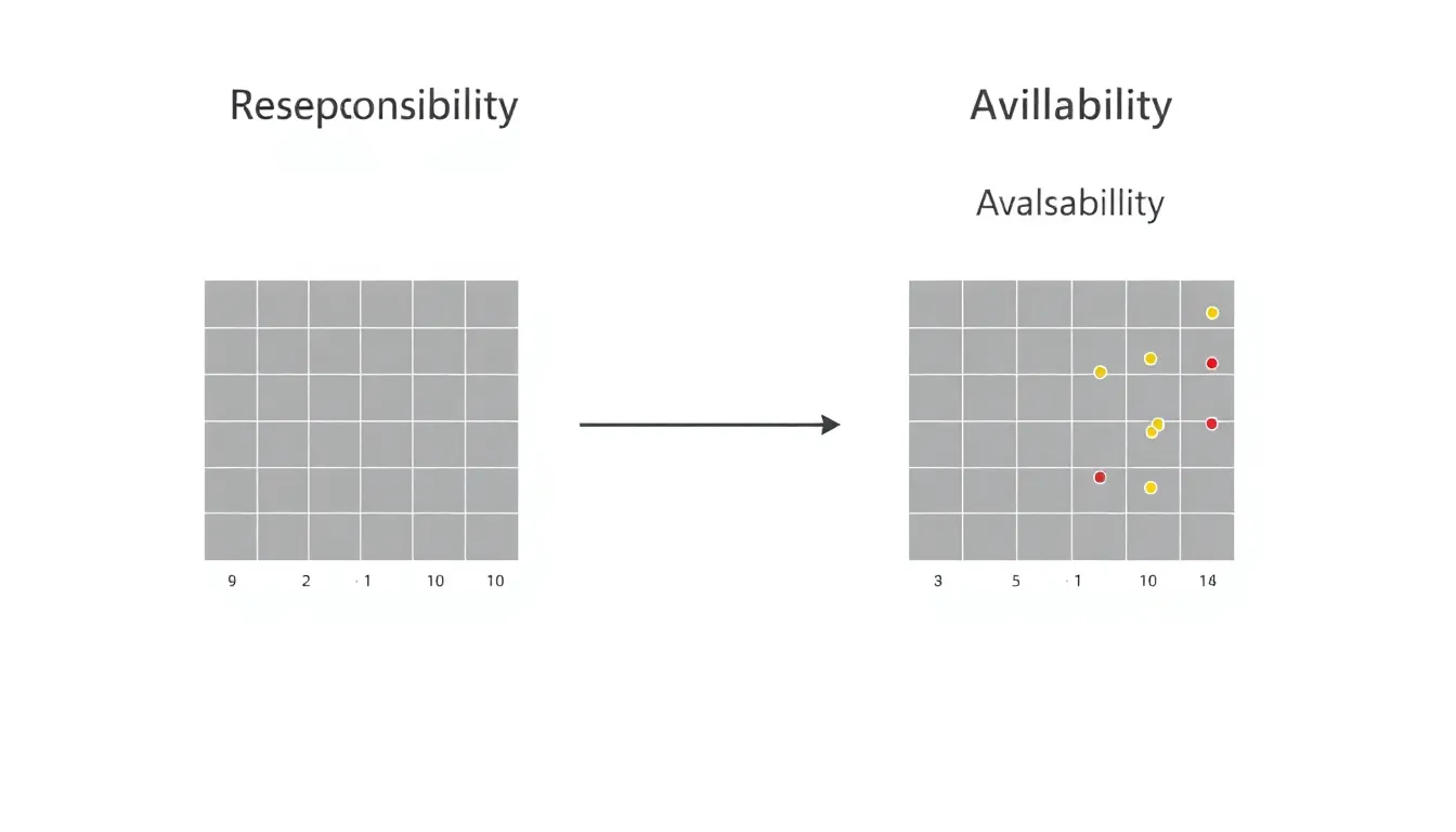
Affinity propagation is a clustering algorithm that takes a fundamentally different approach than traditional methods like k-means. Instead of fixing the number of clusters upfront, it lets the data decide the number of clusters by exchanging messages between data points. These messages represent how well-suited a point is to be an exemplar (cluster center) for another point.
The algorithm operates by iteratively updating two matrices: responsibility and availability. Responsibility reflects how appropriate it is for point k to be the exemplar for point i, while availability reflects how appropriate it is for point i to choose point k as its exemplar. The interplay between these two matrices helps the algorithm converge to a set of exemplars that best represent the data clusters.
One of the most appealing aspects of affinity propagation is that it doesn’t require you to specify the number of clusters beforehand. Instead, you provide a “preference” value for each point, which can be thought of as the a priori suitability of a point to be an exemplar. By tweaking this preference, you can influence the granularity of the clusters, but the algorithm itself finds the optimal exemplar points.
Affinity propagation relies on the concept of “similarity,” which you can define in terms of negative squared Euclidean distance or any other metric that suits your problem domain. The algorithm maximizes the sum of similarities between points and their exemplars, effectively finding a clustering arrangement that maximizes overall similarity within clusters.
Here’s a concise explanation of how the messages update:
For each pair of points (i, k):
  responsibility(i, k) = similarity(i, k) - max_{k' ≠ k} [availability(i, k') + similarity(i, k')]

  availability(i, k) = min{0, responsibility(k, k) + sum_{i' ∉ {i,k}} max(0, responsibility(i', k))}

For k = i:
  availability(k, k) = sum_{i' ≠ k} max(0, responsibility(i', k))
The iterative updates continue until the cluster centers stabilize or a maximum number of iterations is reached. The algorithm’s complexity is roughly O(N²), which can be a limiting factor for very large datasets, but it tends to provide high-quality clusters even when the number of clusters is not known upfront.
Because it uses real-valued similarities and message passing, affinity propagation can capture more nuanced relationships between points than methods that rely on strict geometric constraints. It’s particularly useful when clusters have irregular shapes or when you want a data-driven approach to determining the number of clusters.
Understanding these internal mechanics not only helps you tune the algorithm effectively but also gives insight into why it works better than alternatives in many scenarios. The balance between responsibility and availability can be seen as a negotiation between points about who should represent whom, which is a refreshing perspective compared to centroid-based heuristics.
Next, let’s see what it takes to set up an affinity propagation model using scikit-learn, where you can quickly experiment with this algorithm on your own datasets without getting bogged down in the implementation details. But before that, keep in mind the importance of choosing a proper similarity measure and adjusting the preference parameter to guide the clustering results.

Apple AirTag (2nd Generation): Tracker for Keychain, Wallet, and More; Locator with Sound; Simple One-Tap Setup with iPhone or iPad; Key Finder with up to 1.5X Precision Finding Range
$22.56 (as of October 15, 2026 00:39 GMT +00:00 - More infoProduct prices and availability are accurate as of the date/time indicated and are subject to change. Any price and availability information displayed on [relevant Amazon Site(s), as applicable] at the time of purchase will apply to the purchase of this product.)Setting up your first affinity propagation model in scikit-learn
Scikit-learn provides a simpler interface to affinity propagation through its AffinityPropagation class. To get started, you need to import the class and prepare your data, typically as a NumPy array or a pandas DataFrame. The algorithm expects either a precomputed similarity matrix or raw data points from which it computes negative squared Euclidean distances by default.
Here’s a minimal example using synthetic data to illustrate the workflow:
from sklearn.cluster import AffinityPropagation
from sklearn.datasets import make_blobs
import numpy as np

# Generate sample data with 3 centers
X, _ = make_blobs(n_samples=300, centers=3, cluster_std=0.60, random_state=0)

# Initialize AffinityPropagation with default parameters
af = AffinityPropagation(random_state=42)

# Fit the model
af.fit(X)

# Extract cluster centers and labels
cluster_centers_indices = af.cluster_centers_indices_
labels = af.labels_

print(f"Number of clusters: {len(cluster_centers_indices)}")
print(f"Cluster centers:n{X[cluster_centers_indices]}")
In this example, make_blobs generates a simple dataset with three clusters. The AffinityPropagation instance uses default settings, including the preference parameter set to the median similarity, which often yields a reasonable number of clusters without manual tuning.
After fitting, cluster_centers_indices_ gives the indices of the exemplars within the dataset, and labels_ assigns each point to one of those exemplars. This direct mapping to data points as exemplars is a distinctive feature compared to centroid-based clustering.
If you want to control the number of clusters more explicitly, adjusting the preference parameter is the primary lever. Higher preference values tend to produce more clusters because more points qualify as exemplars, while lower values reduce the number of clusters. Here’s how you might experiment with different preferences:
# Set a high preference to encourage more clusters
high_pref = np.max(-np.sum((X[:, np.newaxis] - X)**2, axis=2))  # max similarity (neg squared distance)

af_high = AffinityPropagation(preference=high_pref, random_state=42)
af_high.fit(X)
print(f"Clusters with high preference: {len(af_high.cluster_centers_indices_)}")

# Set a low preference to encourage fewer clusters
low_pref = np.min(-np.sum((X[:, np.newaxis] - X)**2, axis=2))  # min similarity (neg squared distance)

af_low = AffinityPropagation(preference=low_pref, random_state=42)
af_low.fit(X)
print(f"Clusters with low preference: {len(af_low.cluster_centers_indices_)}")
Notice how you can compute the similarity matrix implicitly by calculating the negative squared Euclidean distances. This approach lets you pick preference values grounded in your data’s distribution, which is more intuitive than arbitrary guesses.
Scikit-learn also allows you to provide a custom similarity matrix directly by setting the affinity parameter to "precomputed". That’s useful if your similarity measure deviates from Euclidean distance or if you want to encode domain-specific relationships.
Here’s how to use a precomputed similarity matrix:
from sklearn.metrics import pairwise_distances

# Compute negative squared Euclidean distances as similarity
similarity = -pairwise_distances(X, metric='sqeuclidean')

af_precomputed = AffinityPropagation(affinity='precomputed', random_state=42)
af_precomputed.fit(similarity)

print(f"Number of clusters (precomputed affinity): {len(af_precomputed.cluster_centers_indices_)}")
In practice, preparing a well-scaled and meaningful similarity matrix can dramatically affect clustering quality. Sometimes, normalizing or transforming your similarities before feeding them in is necessary to emphasize relevant structures.
Affinity propagation also supports parameters like damping, which controls the update rate of messages to avoid oscillations, and max_iter to cap the number of iterations. Tuning these can improve convergence speed and stability, especially on noisy data.
Here’s an example setting a higher damping factor and limiting iterations:
af_tuned = AffinityPropagation(damping=0.9, max_iter=200, random_state=42)
af_tuned.fit(X)
print(f"Clusters with tuned parameters: {len(af_tuned.cluster_centers_indices_)}")
Getting comfortable with these options and experimenting on your datasets is the best way to harness affinity propagation. The scikit-learn implementation abstracts away the complex message-passing mechanics, letting you focus on data and parameter choices.