Handling High-dimensional Data with scipy.sparse.csgraph

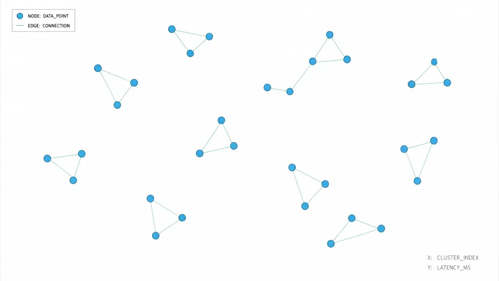
A dense adjacency matrix for a graph with n vertices spends memory on every possible edge, including the ones that do not exist. At four bytes per entry, a matrix for a million vertices would require roughly four terabytes before overhead. Sparse matrices store only nonzero entries and the indexing data needed to find them.

For a graph whose edges are added in batches, build coordinate arrays first: one array for source vertices, one for destinations, and optionally one for weights. A COO matrix is a convenient assembly format; convert it to CSR for fast traversal by row.

import numpy as np
from scipy.sparse import coo_matrix

sources = np.asarray([0, 0, 2, 3], dtype=np.int32)
targets = np.asarray([1, 2, 3, 0], dtype=np.int32)
weights = np.ones(len(sources), dtype=np.uint8)

n = 4
coo = coo_matrix((weights, (sources, targets)), shape=(n, n))
graph = coo.tocsr()

CSR stores three arrays: data contains edge values, indices contains destination vertices, and indptr marks the start of each source vertex’s neighbor range. The neighbors of vertex u are indices[indptr[u]:indptr[u + 1]]. With 32-bit indices and one-byte edge values, storage is approximately five bytes per edge plus four bytes per vertex, ignoring allocator overhead. Use 64-bit indices when vertex counts or nonzero counts can exceed the 32-bit range.

def neighbors(graph, u):
    start = graph.indptr[u]
    end = graph.indptr[u + 1]
    return graph.indices[start:end]

For an undirected graph, each edge generally appears twice, once in each row. Add both directions during construction, or add the transpose before converting to CSR. COO conversion sums duplicate coordinates by default, which is useful when repeated edges represent accumulated weights; for an unweighted graph, duplicates may need to be collapsed back to one.

Choose the value dtype to match the meaning of an edge. Boolean or one-byte values suffice for connectivity; weighted edges need a numeric type with the required range and precision. A zero is treated as absence by many sparse operations, so zero-weight edges need a separate representation or a nonzero marker in the structure. For repeated neighbor scans, CSR’s contiguous row ranges avoid the per-edge object and pointer overhead of a Python list of lists, while

Choosing the right graph structure

while insertions and deletions are rare. CSR is a poor fit when the graph changes constantly: inserting one edge can shift a large suffix of the arrays. If updates are frequent, keep a mutable construction structure such as per-vertex vectors, then periodically compact it into CSR for traversal. The compaction cost is worthwhile only when enough queries reuse the resulting structure.

Match the sparse format to the dominant operation. CSR makes outgoing-neighbor scans efficient. CSC has the same layout organized by destination, so incoming-neighbor scans are efficient. If both directions are hot, keeping both formats costs roughly twice the edge storage but avoids repeatedly transposing or searching. For a directed graph with m edges, building the second index is typically O(n + m); compare that predictable cost with the repeated work it replaces.

from scipy.sparse import csr_matrix

outgoing = csr_matrix((weights, (sources, targets)), shape=(n, n))
incoming = outgoing.tocsc()

def out_neighbors(graph, u):
    a, b = graph.indptr[u], graph.indptr[u + 1]
    return graph.indices[a:b]

def in_neighbors(graph, v):
    a, b = incoming.indptr[v], incoming.indptr[v + 1]
    return incoming.indices[a:b]

A plain edge list is often the better representation when an algorithm processes every edge once and rarely asks for the neighbors of a particular vertex. Two integer arrays for endpoints are compact and sequential to scan, with no per-vertex index array. Sorting edges by source and recording row offsets turns that list into CSR when grouped traversal becomes important.

For graphs that fit comfortably in memory and have many edges per vertex, a dense bit matrix can beat sparse storage for unweighted connectivity. It stores one bit per possible edge rather than a full numeric value and indices for each present edge. The crossover depends on the sparse format’s index widths and value dtype, but for CSR with 32-bit indices and one-byte values, each stored edge costs about five bytes before row pointers. A bit matrix approaches that cost near one edge in forty possible positions; faster bulk operations may justify it at lower densities.

Do not assume that a Python adjacency list is compact because each neighbor is an integer. A list of lists carries a list object per vertex, spare capacity in each list, references for each entry, and Python integer objects unless values are shared or otherwise compacted. It is convenient for irregular dynamic updates and small graphs, but for large static graphs the object overhead can exceed the edge data by an order of magnitude. Typed arrays per vertex reduce the cost, though they still leave one object and allocation per row.

Vertex numbering affects locality. If related vertices receive nearby IDs, rows and destination indices may touch fewer cache lines during traversal. A permutation can improve locality for repeated searches, but it requires remapping every endpoint and any external vertex labels. Measure the full workload: a reordered graph may traverse faster while making construction, updates, or result translation more expensive.

For a workload that needs fast membership tests as well as neighbor iteration, CSR alone is not a constant-time edge lookup structure. A binary search in a sorted row costs O(log degree); an auxiliary hash set can reduce expected lookup time at the cost of substantial memory and less sequential access. The right choice depends on whether edge queries are rare enough to justify searching the row or frequent enough to warrant

Building connectivity without wasting memory

COO is convenient, but it can keep several full-size arrays alive at once: the source coordinates, destination coordinates, values, and the converted CSR arrays. When edges can be read twice, count each row first, allocate the final arrays exactly once, then fill them directly. This avoids the coordinate arrays and the conversion copy.

import numpy as np

def build_csr(n, edges):
    # edges() must return a fresh iterator on each call.
    degree = np.zeros(n, dtype=np.int64)

    for u, v in edges():
        degree[u] += 1

    indptr = np.empty(n + 1, dtype=np.int64)
    indptr[0] = 0
    np.cumsum(degree, out=indptr[1:])

    indices = np.empty(int(indptr[-1]), dtype=np.int32)
    cursor = indptr[:-1].copy()

    for u, v in edges():
        indices[cursor[u]] = v
        cursor[u] += 1

    return indptr, indices

The construction needs one pass to count degrees and another to place destinations. The cursor array advances within each row; after filling, indptr and indices are already a usable CSR representation. Use a 64-bit destination dtype if vertex IDs can exceed the signed 32-bit range. For weighted edges, allocate a matching data array and write each weight at the same cursor position as its destination.

For an undirected graph, count and write both directions for each input edge. Decide explicitly how self-loops and duplicate edges should behave: emitting both directions for a self-loop stores it twice, and direct filling does not automatically combine duplicates. If duplicates are invalid, reject them during ingestion or sort each row and remove repeated destinations in a separate pass; otherwise, repeated entries may cause neighbor scans to process the same connection more than once.

If the input cannot be replayed, spool compact endpoint arrays to disk or retain a compact edge list for the second pass. Avoid saving edges as Python tuples: object headers and references can outweigh the endpoint values. Fixed-width arrays keep the temporary representation predictable, and

Finding paths through high-dimensional data

avoid a second full-size copy of the graph. When memory is tight, construct rows in chunks, write each completed chunk to a memory-mapped array, or use a two-pass input source rather than retaining both a Python representation and the final index.

In high-dimensional data, a graph often represents local similarity rather than an explicitly observed network. Each point becomes a vertex, and edges connect it to nearby points. The tempting construction is to compute every pairwise distance and keep the smallest values in each row. That requires quadratic storage if the full distance matrix is materialized, and roughly O(N²D) distance work for N points with D coordinates. Keep only the selected neighbors, not the intermediate matrix.

For modest datasets, process points in batches against the full collection, discard each batch’s distance matrix after selecting its nearest neighbors, and append only the resulting endpoints and distances. For large datasets, approximate nearest-neighbor indexes reduce the candidate set before exact distances are evaluated. The index is a search structure for graph construction; the finished graph can still be stored as CSR for traversal.

import numpy as np
from sklearn.neighbors import NearestNeighbors

# X has shape (number of points, number of dimensions).
k = 12
search = NearestNeighbors(
    n_neighbors=k + 1,
    algorithm="auto",
    metric="euclidean",
).fit(X)

distances, neighbors = search.kneighbors(X)

# The first result is normally the point itself.
sources = np.repeat(np.arange(X.shape[0]), k)
targets = neighbors[:, 1:].reshape(-1)
weights = distances[:, 1:].reshape(-1)

Nearest-neighbor relations are generally directed: point u may select v without v selecting u. For an undirected graph, choose a rule deliberately. The union rule keeps an edge if either endpoint selects the other; the mutual rule keeps it only if both do. Union tends to preserve connectivity, while mutual selection suppresses asymmetric links that may cross a sparse region.

from scipy.sparse import coo_matrix

n = X.shape[0]
directed = coo_matrix(
    (weights, (sources, targets)),
    shape=(n, n),
).tocsr()

# Union of directed neighbor relations. Keep the smaller distance
# when both directions produced the same pair.
undirected = directed.minimum(directed.T)
undirected = directed.maximum(directed.T)

For distance weights, the union operation needs care: taking the elementwise maximum of a distance matrix selects the larger distance where both directions exist. A robust approach is to combine a sparse matrix with its transpose using an explicit reduction, or to canonicalize undirected endpoint pairs before building CSR. For similarity weights, maximum may be the intended rule; for distances, minimum is often appropriate. The meaning of the values determines the operation.

Once the graph is built, breadth-first search answers reachability and minimum-edge-count questions on an unweighted graph. Dijkstra’s algorithm answers minimum-total-cost questions when edge values are nonnegative costs. Keep the two meanings separate: a distance stored as an edge cost does not make a BFS path distance-weighted.

from scipy.sparse.csgraph import breadth_first_order, dijkstra

source = 0

order, predecessors = breadth_first_order(
    undirected,
    i_start=source,
    directed=False,
    return_predecessors=True,
)

costs, weighted_predecessors = dijkstra(
    undirected,
    directed=False,
    indices=source,
    return_predecessors=True,
)

A predecessor array encodes paths without storing a separate path object for every reached vertex. To recover one path, follow predecessors backward from the destination, then reverse the collected vertex IDs. An unreachable vertex has a sentinel predecessor, so test reachability before reconstruction.

def recover_path(predecessors, source, destination):
    path = []
    vertex = destination

    while vertex != source:
        if vertex < 0 or predecessors[vertex] < 0:
            return None
        path.append(int(vertex))
        vertex = int(predecessors[vertex])

    path.append(int(source))
    path.reverse()
    return path

path = recover_path(weighted_predecessors, source, destination)

High-dimensional distance measures can lose contrast: the nearest and farthest points may become nearly equally distant, making a fixed neighbor count less meaningful. Check the distribution of selected edge lengths and the number of connected components. A graph with many isolated components cannot provide paths between them, regardless of how efficient the search routine is. If local scales vary substantially, normalize edge distances by a per-vertex scale before comparing paths, or

Measuring performance and checking results

use a locally scaled similarity rather than a raw distance threshold. Before tuning the path search, measure the graph that the search will actually traverse: vertex count, edge count, degree distribution, connected components, and edge-value range. These properties often explain runtime more directly than the original feature dimension.

Benchmark construction and queries separately. Include input conversion in construction timings only if production will perform that conversion; otherwise the measurement answers the wrong question. Warm up code paths, run several trials, and report the median rather than the fastest sample. Keep the graph and query set fixed between implementations.

from time import perf_counter
import numpy as np

def median_seconds(fn, repeats=7):
    fn()  # warm up
    samples = []

    for _ in range(repeats):
        start = perf_counter()
        fn()
        samples.append(perf_counter() - start)

    return float(np.median(samples))

build_time = median_seconds(lambda: build_graph())
search_time = median_seconds(lambda: run_queries(graph, queries))

print(f"build: {build_time:.6f} s")
print(f"queries: {search_time:.6f} s")

Do not time a function that returns a large result and then immediately discard it if production must retain that result. Conversely, if only aggregate answers are needed, accumulate them inside the timed operation so allocation and result materialization are represented consistently. Separate one-time index construction from repeated query time; the break-even point is approximately the construction cost divided by the per-query savings.

Record memory as well as elapsed time. Array payload sizes are easy to inspect, but they omit allocator overhead and temporary copies. For CSR, account for all three arrays; a second orientation, such as CSC, is additional storage rather than a free view.

def csr_payload_bytes(graph):
    return (
        graph.data.nbytes
        + graph.indices.nbytes
        + graph.indptr.nbytes
    )

print(f"CSR payload: {csr_payload_bytes(graph) / 2**20:.1f} MiB")
print(f"vertices: {graph.shape[0]}")
print(f"stored entries: {graph.nnz}")

Check the graph before trusting a fast result. Confirm that endpoint IDs are in range, that row offsets are monotonic, and that the final offset equals the number of stored entries. For an undirected graph, verify symmetry on a manageable sample or compare the structure with its transpose. If duplicates are forbidden, ensure that each sorted row contains no repeated destination.

def validate_csr(indptr, indices, n):
    assert len(indptr) == n + 1
    assert indptr[0] == 0
    assert np.all(indptr[1:] >= indptr[:-1])
    assert indptr[-1] == len(indices)
    assert np.all(indices >= 0)
    assert np.all(indices < n)

    for u in range(n):
        row = indices[indptr[u]:indptr[u + 1]]
        assert np.all(row[1:] >= row[:-1])
        assert len(row) == len(np.unique(row))

Validation itself can be expensive on a large graph, so run full checks during construction tests and use sampled rows or aggregate invariants in production. For a small graph, compare the sparse implementation against a simple reference representation. Small exhaustive cases expose errors in duplicate handling, self-loops, directionality, and unreachable-path behavior more reliably than a large random benchmark.

def reference_neighbors(edges, n):
    result = [set() for _ in range(n)]
    for u, v in edges:
        result[u].add(v)
    return result

reference = reference_neighbors(edge_list, n)

for u in range(n):
    actual = set(map(int, neighbors(graph, u)))
    assert actual == reference[u]

Path algorithms need result checks beyond runtime. For each returned path, verify that consecutive vertices are connected by stored edges and that the reported cost equals the sum of their edge weights. For unweighted BFS, compare path length against a reference search on small graphs. Include disconnected graphs and vertices with empty rows; these are ordinary cases, not exceptional conditions.

Measure representative queries rather than repeatedly searching from one unusually well-connected source. Sources with different component sizes and degree patterns can produce very different traversal work. Track visited vertices and examined edges alongside elapsed time: if those counts change between runs, the timings are not measuring equivalent workloads.