Advanced Signal Filtering with scipy.signal

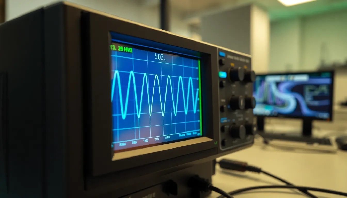
Signal processing, at its core, is about manipulating or analyzing signals to extract useful information or to transform them in a desired way. Whether you are dealing with audio, sensor data, or any time-series information, the fundamental concepts remain consistent.

One of the key ideas is the representation of signals as functions, often discrete sequences in digital signal processing. This means we consider a signal as a series of samples taken at uniform intervals—each sample representing the signal’s amplitude at a particular moment.

Consider a simple sine wave, which is the building block for more complex signals. Generating a sine wave in Python is simpler using NumPy:

import numpy as np
import matplotlib.pyplot as plt

fs = 500  # Sampling frequency in Hz
t = np.arange(0, 1, 1/fs)  # Time vector for 1 second
f = 5  # Frequency of the sine wave in Hz
signal = np.sin(2 * np.pi * f * t)

plt.plot(t, signal)
plt.title("5 Hz Sine Wave")
plt.xlabel("Time [s]")
plt.ylabel("Amplitude")
plt.show()

This snippet creates a 5 Hz sine wave sampled at 500 Hz. The sampling frequency (fs) must be at least twice the highest frequency component of the signal to satisfy the Nyquist criterion and avoid aliasing.

Another concept that often trips people up is the difference between time domain and frequency domain. Time domain is how the signal changes over time, but the frequency domain shows the constituent frequencies. To move from one to the other, we use the Fourier transform.

Here’s how to compute and visualize the frequency spectrum of the sine wave:

from numpy.fft import fft, fftfreq

n = len(signal)
yf = fft(signal)
xf = fftfreq(n, 1/fs)

plt.stem(xf[:n//2], np.abs(yf[:n//2]), use_line_collection=True)
plt.title("Frequency Spectrum")
plt.xlabel("Frequency [Hz]")
plt.ylabel("Magnitude")
plt.show()

The Fourier transform breaks the signal down into components of different frequencies, showing peaks at the frequencies present—in this case, prominently at 5 Hz. The magnitude of the FFT output tells you the strength of each frequency component.

Understanding convolution is also pivotal. Convolution allows you to apply filters to signals by combining the signal with an impulse response. In discrete time, convolution sums this product of the input signal and the filter’s coefficients shifted over time.

Here’s a quick example of convolving a signal with a simple moving average filter:

filter_size = 5
moving_average_filter = np.ones(filter_size) / filter_size
smoothed_signal = np.convolve(signal, moving_average_filter, mode='same')

plt.plot(t, signal, label='Original')
plt.plot(t, smoothed_signal, label='Smoothed')
plt.legend()
plt.show()

This moving average filter reduces high-frequency noise by averaging neighboring samples, effectively smoothing the signal. The ‘mode’ parameter ensures the output signal has the same length as the input.

Before jumping into more advanced filtering techniques, it’s essential to grasp these basics—sampling, frequency representation, and convolution. They form the foundation for understanding how digital filters work and how to process signals effectively.

One common pitfall is misunderstanding the impact of filter length and type. For instance, FIR (Finite Impulse Response) filters have a finite number of coefficients and are inherently stable, while IIR (Infinite Impulse Response) filters use feedback and can achieve sharper frequency responses with fewer coefficients but may become unstable if not designed carefully.

In Python, the scipy.signal module provides robust tools to design and apply these filters, but before using those, you should be comfortable with manually implementing simple filters and interpreting their effects.

Let’s peek at a basic FIR filter design using a window method:

from scipy.signal import firwin, lfilter

numtaps = 31  # Number of filter coefficients (filter length)
cutoff = 0.1  # Normalized cutoff frequency (Nyquist = 1)

fir_coeff = firwin(numtaps, cutoff)
filtered_signal = lfilter(fir_coeff, 1.0, signal)

plt.plot(t, signal, label='Original')
plt.plot(t, filtered_signal, label='Filtered')
plt.legend()
plt.show()

This FIR filter acts as a low-pass filter, allowing frequencies below the cutoff to pass while attenuating higher frequencies. The firwin function uses windowing techniques to generate the filter coefficients.

These building blocks—understanding sampling, the frequency domain, convolution, and basic filter design—are what you need to master before exploring the more advanced tools that the scipy.signal module offers to tackle real-world signals.

Once you’re comfortable with these fundamentals, you can start experimenting with other filter types, adaptive filters, and spectral estimation methods that can handle noise and non-stationary signals more effectively. But that, as they say, is a story for next time when we dive into the real power of scipy.signal and its advanced filtering capabilities.

Before moving on, remember that signal processing is as much art as science. The choices you make in sampling, windowing, and filter design all influence the final result, so understanding the trade-offs is key. For example, longer filters have better frequency resolution but introduce more delay, which can be problematic in real-time applications.

Also, keep in mind that numerical issues can creep in. Finite precision arithmetic, especially with IIR filters, might cause instability or unexpected behavior. Running simulations and visualizing results—like we’ve done here—is invaluable for diagnosing and correcting such problems.

With this foundation laid out, you’re ready to tackle the next level: how to harness the full feature set of scipy.signal to design sophisticated filters, perform spectral analysis, and optimize your code for large datasets. But first, let’s explore some of the more advanced filtering techniques that go beyond simple moving averages and basic FIR filters.

For example, consider the Butterworth filter, which is popular for its flat passband. Designing one is straightforward:

from scipy.signal import butter, filtfilt

order = 4
cutoff_freq = 0.1  # Normalized frequency (Nyquist = 1)
b, a = butter(order, cutoff_freq, btype='low')

filtered_signal = filtfilt(b, a, signal)  # Zero-phase filtering

plt.plot(t, signal, label='Original')
plt.plot(t, filtered_signal, label='Butterworth Filtered')
plt.legend()
plt.show()

The use of filtfilt applies the filter forward and backward to eliminate phase distortion, which is important in applications where phase information matters, like audio or biomedical signals.

Another point worth mentioning is that the normalized cutoff frequency is expressed relative to the Nyquist frequency, which is half the sampling rate. So, if your sampling rate changes, all cutoff parameters must be adjusted accordingly.

To summarize: start with representing signals correctly, understand the frequency domain with FFT, apply simple filters like moving averages to get a feel for convolution, and then explore digital filter design with FIR and IIR filters. Each step builds on the last, setting you up to apply the powerful tools available in scipy.signal confidently and effectively.

Next, we’ll see how to leverage these techniques to tackle more challenging filtering problems, including noise reduction and signal enhancement, but for now, that is the groundwork you need to truly understand what’s happening under the hood.

Let’s keep going—

Exploring advanced filtering techniques with scipy.signal

Building on the Butterworth example, you might want to explore other classic IIR filters like Chebyshev or Elliptic filters, which trade off ripple in the passband or stopband for steeper roll-off. Here’s how you design and apply a Chebyshev Type I filter:

from scipy.signal import cheby1, filtfilt

order = 4
rp = 1  # Passband ripple in dB
cutoff_freq = 0.1

b, a = cheby1(order, rp, cutoff_freq, btype='low')
filtered_signal = filtfilt(b, a, signal)

plt.plot(t, signal, label='Original')
plt.plot(t, filtered_signal, label='Chebyshev Type I Filtered')
plt.legend()
plt.show()

Notice how the rp parameter controls the allowable ripple in the passband, which is a key design choice. The steeper roll-off can be beneficial when you need to sharply separate frequency bands but at the cost of some passband variation.

Another powerful tool in scipy.signal is the use of bandpass and bandstop filters. These are invaluable when you want to isolate or remove specific frequency bands, for example, eliminating 60 Hz power line noise in biomedical signals. Here’s how you can create a bandstop (notch) filter to attenuate a narrow frequency range:

from scipy.signal import iirnotch

fs = 500  # Sampling frequency
f0 = 60.0  # Frequency to remove from signal (Hz)
Q = 30.0  # Quality factor

w0 = f0 / (fs / 2)  # Normalized Frequency
b, a = iirnotch(w0, Q)
filtered_signal = filtfilt(b, a, signal)

plt.plot(t, signal, label='Original')
plt.plot(t, filtered_signal, label='Notch Filtered (60 Hz)')
plt.legend()
plt.show()

The quality factor Q controls the bandwidth of the notch; higher Q means a narrower notch. This approach is essential in cleaning up signals contaminated by narrowband interference.

Moving beyond classical filters, wavelet transforms offer a time-frequency decomposition that adapts better to non-stationary signals. While scipy.signal has limited wavelet functionality, the pywt library complements it well for this purpose. Here’s a quick example of denoising a signal using discrete wavelet transform:

import pywt

coeffs = pywt.wavedec(signal, 'db4', level=4)
threshold = 0.2
coeffs_thresh = [pywt.threshold(c, threshold, mode='soft') for c in coeffs]
denoised_signal = pywt.waverec(coeffs_thresh, 'db4')

plt.plot(t, signal, label='Original')
plt.plot(t[:len(denoised_signal)], denoised_signal, label='Denoised')
plt.legend()
plt.show()

This method preserves signal features better than traditional low-pass filtering when noise is spread across frequencies or transient in nature.

Another advanced filtering technique is adaptive filtering, where filter coefficients change over time to track signal variations or noise characteristics. Although scipy.signal doesn’t provide built-in adaptive filters, implementing algorithms like LMS (Least Mean Squares) or RLS (Recursive Least Squares) is simpler and worth exploring when dealing with real-time or non-stationary signals.

Here is a minimal LMS adaptive filter example:

import numpy as np

def lms_filter(desired, input_signal, mu, filter_order):
    n_samples = len(input_signal)
    weights = np.zeros(filter_order)
    output = np.zeros(n_samples)
    error = np.zeros(n_samples)

    for n in range(filter_order, n_samples):
        x = input_signal[n-filter_order:n][::-1]
        y = np.dot(weights, x)
        e = desired[n] - y
        weights += 2 * mu * e * x
        output[n] = y
        error[n] = e

    return output, error, weights

# Simulated example: desired is the clean signal, input_signal is noisy
mu = 0.01
filter_order = 10
noisy_signal = signal + 0.5 * np.random.randn(len(signal))
output, error, weights = lms_filter(signal, noisy_signal, mu, filter_order)

plt.plot(t, noisy_signal, label='Noisy Input')
plt.plot(t, output, label='LMS Filter Output')
plt.legend()
plt.show()

Adaptive filters shine when noise characteristics change over time, as they continually update their parameters to minimize the error between the output and the desired signal.

Finally, spectral estimation techniques such as the Welch method or multitaper method allow you to estimate power spectral density more robustly, especially for noisy or short-duration signals. Here’s how to compute a Welch power spectral density estimate:

from scipy.signal import welch

fs = 500
frequencies, psd = welch(signal, fs, nperseg=256)

plt.semilogy(frequencies, psd)
plt.title('Power Spectral Density using Welch Method')
plt.xlabel('Frequency [Hz]')
plt.ylabel('PSD [V**2/Hz]')
plt.show()

The Welch method reduces variance of the spectral estimate by averaging periodograms computed on overlapping segments of the signal.

Each of these advanced tools—designing sharper filters, notch filtering, wavelet denoising, adaptive filtering, and spectral estimation—equips you to tackle complex real-world signal processing challenges. As you integrate them into your workflows, the key is to understand their assumptions, limitations, and how parameter choices impact your results.

Next up, we’ll delve into strategies for optimizing performance when processing large datasets, ensuring your algorithms run efficiently without sacrificing accuracy, but before that, consider experimenting with these techniques on your own signals to see how they behave in practice.

Optimizing performance for large-scale signal analysis

When dealing with large-scale signal analysis, efficiency becomes paramount. Processing large datasets can quickly lead to performance bottlenecks if not handled correctly. Python, coupled with libraries like NumPy and SciPy, provides a rich ecosystem for signal processing, but you must also be mindful of how you structure your code and data to optimize for speed and memory usage.

One fundamental approach to enhancing performance is to leverage vectorized operations. Instead of using Python loops to process individual elements, you can take advantage of NumPy’s ability to perform operations on entire arrays concurrently. This not only speeds up your code but also makes it more readable. For example, consider the following code that applies a simple operation to a large signal:

import numpy as np

# Simulating a large signal
signal_length = 10**6
signal = np.random.rand(signal_length)

# Vectorized operation: scaling the signal
scaled_signal = signal * 2.5

In this snippet, the scaling operation is applied to the entire signal array in one go, which is significantly faster than iterating through each sample.

Another common technique is to use efficient memory management practices. When working with large datasets, ensure you’re using data types that consume less memory. For instance, if your signal data can be represented as floats, consider using float32 instead of the default float64:

signal = np.random.rand(signal_length).astype(np.float32)

This change can halve the memory usage, which is critical when working with millions of samples.

For more complex operations, consider using the numba library, which allows you to compile Python functions to machine code at runtime. This can lead to significant speed improvements, especially for functions that are computationally intensive. Here’s a simple example of using Numba to accelerate a custom filter function:

from numba import jit

@jit(nopython=True)
def apply_filter(signal, filter_coeffs):
    n_samples = len(signal)
    filtered_signal = np.zeros(n_samples)
    for n in range(len(filter_coeffs), n_samples):
        filtered_signal[n] = np.dot(filter_coeffs, signal[n-len(filter_coeffs)+1:n+1])
    return filtered_signal

# Example usage
filter_coeffs = np.array([0.2, 0.5, 0.2])
filtered_signal = apply_filter(signal, filter_coeffs)

This decorator @jit(nopython=True) tells Numba to compile the function for maximum speed, which can be a game changer for performance-critical applications.

Parallel processing is another avenue worth exploring. Python’s concurrent.futures module allows you to run computations in parallel, taking advantage of multiple CPU cores. This is particularly useful for independent operations on segments of a large signal. Here’s how you can use it:

from concurrent.futures import ProcessPoolExecutor

def process_segment(segment):
    # Perform some processing on the segment
    return np.mean(segment)

# Split signal into chunks
num_chunks = 10
chunks = np.array_split(signal, num_chunks)

with ProcessPoolExecutor() as executor:
    results = list(executor.map(process_segment, chunks))

# Combine results
mean_values = np.array(results)

In this example, the signal is divided into chunks, and each chunk is processed in parallel. This can drastically cut down on processing time for large datasets.

Don’t forget to consider the computational complexity of the algorithms you’re employing. For instance, using the Fast Fourier Transform (FFT) instead of the naive DFT can reduce the complexity from O(N^2) to O(N log N). This is particularly important when analyzing large signals where performance could otherwise be prohibitive:

from numpy.fft import rfft

# Using FFT for frequency analysis
frequencies = rfft(signal)

Lastly, profiling your code is essential to identify bottlenecks. Python has several profiling tools available, such as cProfile, which can help you pinpoint where your program spends the most time and allow you to focus your optimization efforts effectively:

import cProfile

def main():
    # Your signal processing code here
    pass

cProfile.run('main()')

By applying these performance optimization strategies—leveraging vectorization, efficient memory usage, just-in-time compilation with Numba, parallel processing, and algorithmic efficiency—you can significantly enhance the performance of your signal processing applications. These practices will enable you to handle larger datasets and more complex analyses without sacrificing execution speed or accuracy.